天然地震
OBSpy教程之获取到时
09月08日18时04分在山东青岛市崂山区海域(北纬35.96度,东经120.82度)发生3.0级地震,震源深度13千米。(@中国地震台网)
这里我们使用OBSpy获取上海某台站记录的此地震波形。
1
2
3
4
5
6
7
8
9
10
11
12
13
14
15
16
17
18
19
20
| import obspy
from obspy.clients.fdsn import Client
import os
import numpy as np
import matplotlib.pyplot as plt
event_time = obspy.UTCDateTime("2020-09-08T10:04:44.5")
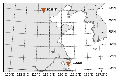
inv = c_event.get_stations(network="IC",
station="BJT",
level="response")
inv.extend(c_event.get_stations(network="IC",
station="SSE",
level="response"))
client = Client("IRIS")
st = client.get_waveforms(network="IC",
station="*",
location="*",
channel="BH*",
starttime=event_time - 10 * 60,
endtime=event_time + 10 * 60)
st.write('./QingDaoEvent20200908/QDshock.mseed')
|
1
2
3
4
5
6
7
8
9
| 25 Trace(s) in Stream:
IC.BJT.00.BH1 | 2020-09-08T09:54:44.519539Z - 2020-09-08T10:14:44.469539Z | 20.0 Hz, 24000 samples
...
(23 other traces)
...
IC.QIZ.00.BHZ | 2020-09-08T09:54:44.519538Z - 2020-09-08T10:14:44.469538Z | 20.0 Hz, 24000 samples
[Use "print(Stream.__str__(extended=True))" to print all Traces]
|
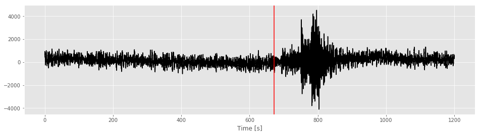
台网:IC,共获取了25道记录,以位于北京白家疃的BJT台站数据为例,计算地震波到达此站的UTC时并将P波到时绘制在图上。
1
2
3
4
5
6
7
8
9
10
11
12
13
14
15
16
17
18
19
20
21
22
23
24
25
26
27
| from obspy.taup import TauPyModel
from obspy.geodetics import locations2degrees
m = TauPyModel(model="ak135", verbose=True)
st = st.select(station="BJT")
Trace = 0
qd_event_latitude = 35.96
qd_event_longitude = 120.82
qd_event_depth = 13
coords = {"longitude":116.1679,
"latitude": 40.0183}
distance = locations2degrees(qd_event_latitude,
qd_event_longitude,
coords["latitude"],
coords["longitude"])
arrivals = m.get_ray_paths(distance_in_degree=distance,
source_depth_in_km=qd_event_depth)
first_arrival = event_time + arrivals[0].time
delta = first_arrival - st[Trace].stats.starttime
time = np.arange(0, st[Trace].stats.npts/ st[Trace].stats.sampling_rate, st[Trace].stats.delta)
fig, axes = plt.subplots(nrows = 1, ncols = 1 , figsize = (16,4))
axes.plot(time, st[Trace].data, color = 'black')
axes.axvline(delta, color = 'red')
axes.set_xlabel("Time [s]"+st[Trace].stats.channel)
|