Receiver Function profile with rf package 此ipynb脚本借助rf软件包 使用智利北部的IPOC数据演示了receiver function的计算和剖面叠加。此脚本依赖项ObsPy,rf,h5py,obspyh5和tqdm。首先,我们导入必要的函数,并为目录,地震和波形文件定义文件名。
1
2
3
4
5
6
7
8
9
10
11
12
13
14
15
16
17
18
19
20
21
import osimport matplotlib.pyplot as pltimport numpy as npfrom obspy import read_inventory, read_events, UTCDateTime as UTCfrom obspy.clients.fdsn import Clientfrom rf import read_rf, RFStreamfrom rf import get_profile_boxes, iter_event_data, IterMultipleComponentsfrom rf.imaging import plot_profile_mapfrom rf.profile import profilefrom tqdm import tqdm""" 创建->data文件夹并定义文件名称 """ data = os.path.join('data' , '' ) invfile = data + 'rf_profile_stations.xml' catfile = data + 'rf_profile_events.xml' datafile = data + 'rf_profile_data.h5' rffile = data + 'rf_profile_rfs.h5' profilefile = data + 'rf_profile_profile.h5' if not os.path.exists(data): os.mkdir(data)
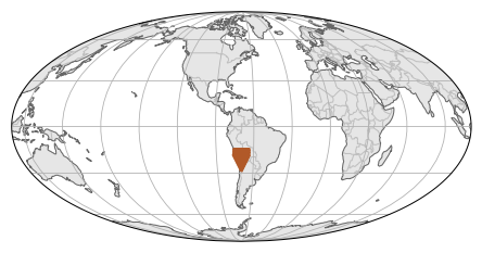
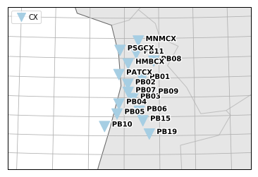
如有必要,可以下载震级5.5和6.5之间的2010年库存数据和事件并作图。
1
2
3
4
5
6
7
8
if not os.path.exists(invfile): client = Client('GFZ' ) inventory = client.get_stations(network='CX' , channel='BH?' , level='channel' , minlatitude=-24 , maxlatitude=-19 ) inventory.write(invfile, 'STATIONXML' ) inventory = read_inventory(invfile) inventory.plot(label=False ) fig = inventory.plot('local' , color_per_network=True )
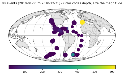
1
2
3
4
5
6
7
8
9
10
11
12
coords = inventory.get_coordinates('CX.PB01..BHZ' ) lonlat = (coords['longitude' ], coords['latitude' ]) if not os.path.exists(catfile): client = Client() kwargs = {'starttime' : UTC('2010-01-01' ), 'endtime' : UTC('2011-01-01' ), 'latitude' : lonlat[1 ], 'longitude' : lonlat[0 ], 'minradius' : 30 , 'maxradius' : 90 , 'minmagnitude' : 5.5 , 'maxmagnitude' : 6.5 } catalog = client.get_events(**kwargs) catalog.write(catfile, 'QUAKEML' ) catalog = read_events(catfile) fig = catalog.plot(label=None )
iter_event_data迭代器下载波形数据,并将其保存到HDF5文件中。 迭代器通过应用rfstats函数自动将必要的标头插入流中。
1
2
3
4
5
6
7
if not os.path.exists(datafile): client = Client('GFZ' ) stream = RFStream() with tqdm() as pbar: for s in iter_event_data(catalog, inventory, client.get_waveforms, pbar=pbar): stream.extend(s) stream.write(datafile, 'H5' )
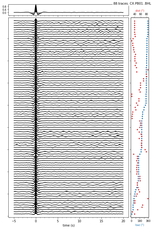
IterMultipleComponents对其进行遍历。 该迭代器为每个事件和台站返回一个三分量流。 我们过滤数据,相对于P波起始点进行修剪,计算接收函数并应用Ps偏移校正。 此后,绘制一个站的L分量和某些站的Q分量。 接收函数的L分量在0s处显示预期的峰值。
1
2
3
4
5
6
7
8
9
10
11
12
data = read_rf(datafile, 'H5' ) stream = RFStream() for stream3c in tqdm(IterMultipleComponents(data, 'onset' , 3 )): stream3c.filter ('bandpass' , freqmin=0.5 , freqmax=2 ) stream3c.trim2(-25 , 75 , 'onset' ) if len (stream3c) != 3 : continue stream3c.rf() stream3c.moveout() stream.extend(stream3c) stream.write(rffile, 'H5' ) print (stream)
1
2
3
4
5
6
7
8
9
3273 Trace(s) in Stream: Prf CX.HMBCX..BHT | -25.0s - 75.0s onset:2010-01-27T17:52:02.949998Z | 20.0 Hz, 2001 samples | mag:5.8 dist:53.1 baz:92.8 slow:6.40 (Ps moveout) ... (3271 other traces) ... Prf CX.PSGCX..BHL | -25.0s - 75.0s onset:2010-12-31T16:39:31.150000Z | 20.0 Hz, 2001 samples | mag:5.5 dist:47.7 baz:70.2 slow:6.40 (Ps moveout) [Use "print(Stream.__str__(extended=True))" to print all Traces]
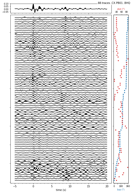
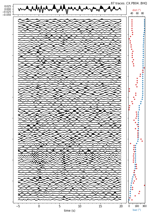
1
2
3
4
5
6
stream = read_rf(rffile, 'H5' ) kw = {'trim' : (-5 , 20 ), 'fillcolors' : ('black' , 'gray' ), 'trace_height' : 0.1 } stream.select(component='L' , station='PB01' ).sort(['back_azimuth' ]).plot_rf(**kw) for sta in ('PB01' , 'PB04' ): stream.select(component='Q' , station=sta).sort(['back_azimuth' ]).plot_rf(**kw) plt.show()
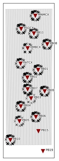
get_profile_boxes函数用于定义要叠加的区域。 方位角为90度,以定义东西走向。 使用plot_profile_map绘制域。 该剖面由配置剖面函数生成。 使用剖面函数而不是RFStream.profile方法可以显示进度条(对于大型数据集,也可以直接从光盘中feedRF数据)。
1
2
3
4
5
6
7
8
9
stream = read_rf(rffile, 'H5' ) ppoints = stream.ppoints(70 ) boxes = get_profile_boxes((-21.3 , -70.7 ), 90 , np.linspace(0 , 180 , 73 ), width=530 ) plt.figure(figsize=(10 , 10 )) plot_profile_map(boxes, inventory=inventory, ppoints=ppoints) pstream = profile(tqdm(stream), boxes) pstream.write(profilefile, 'H5' ) plt.show() print (pstream)
1
2
3
4
5
6
7
8
9
213 Trace(s) in Stream: Prf profile (L) | -25.0s - 75.0s | 20.0 Hz, 2001 samples | pos:1.25km slow:6.40 (Ps moveout) ... (211 other traces) ... Prf profile (T) | -25.0s - 75.0s | 20.0 Hz, 2001 samples | pos:178.75km slow:6.40 (Ps moveout) [Use "print(Stream.__str__(extended=True))" to print all Traces]
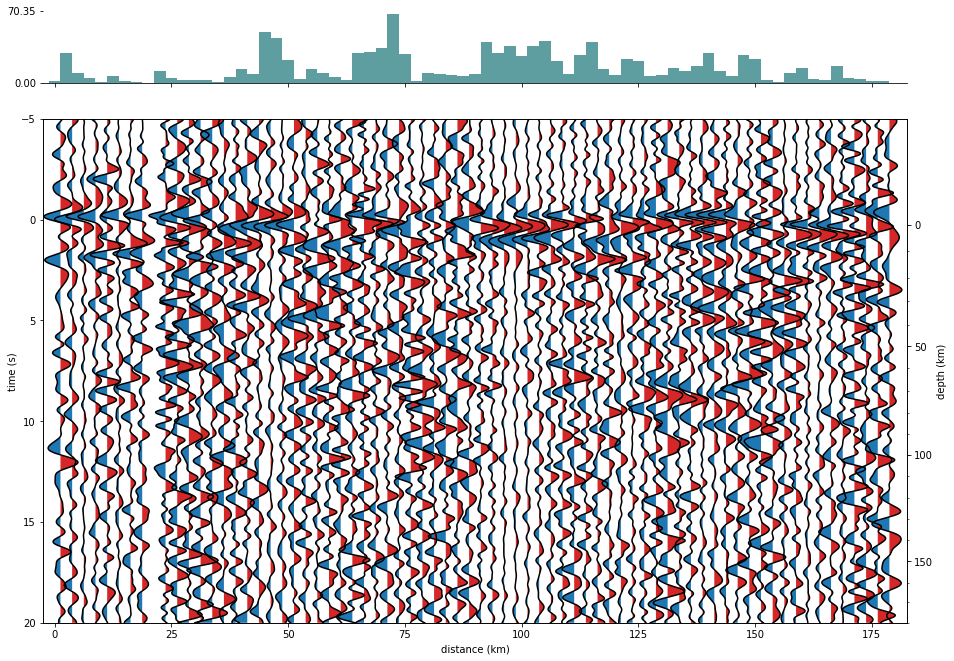
1
2
3
4
5
pstream = read_rf(profilefile) pstream.trim2(-5 , 20 , 'onset' ) pstream.select(channel='??Q' ).normalize().plot_profile(scale=1.5 , top='hist' ) plt.gcf().set_size_inches(15 , 10 ) plt.show()